Introduction
Even as global climate models reach resolutions of a few kilometers (see figure 1), they still struggle to represent turbulence, i.e. chaotic fluid motion, in the lowest part of the atmosphere — the boundary layer. That’s where many of the key interactions between Earth’s surface and the atmosphere happen, and it’s where traditional models fall short due to their inability to resolve small-scale eddies and sharp gradients directly. These models use simplified formulas, called parameterizations, to estimate how turbulence moves heat, moisture, and air near the ground. But these shortcuts often miss important details like the mix of forests, cities, and open land, or how turbulence changes between day and night. As a result, the models can make consistent mistakes in predicting temperature, humidity, and wind near the surface.
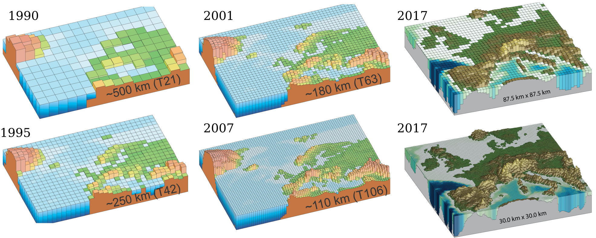
Fig. 1 - Climate model resolution development since 1990. Horizontal resolution of climate models illustrated through their depiction of European topography. Shown are examples from successive IPCC Assessment Reports: First AR (1990), Second AR (1995), Third AR (2001), AR4 (2007, [1]), and AR5 (2017, [2]).
One approach that avoids these modeling assumptions altogether is Direct Numerical Simulation (DNS), which resolves all spatial and temporal scales of motion in a fluid flow — from the smallest turbulent eddies to the largest flow structures. This, however, comes at an enormous computational cost. The key challenge lies in the Reynolds number (Re), a dimensionless quantity characterizing the ratio of inertial to viscous forces in a flow. As the Reynolds number increases, the range of active scales in the flow widens significantly. To fully resolve all turbulent scales in three dimensions, the number of spatial grid points required scales as
\[N = N_x \times N_y \times N_z \sim Re^{9/4},\]i.e. stronger than quadratically!
This steep scaling arises because the smallest scales (Kolmogorov scales) shrink with increasing Re, and resolving them in all three spatial dimensions demands increasingly finer numerical meshes. Moreover, the time-stepping scheme must capture the fastest (smallest-scale) dynamics, which further multiplies the cost. Figure 2 provides an overview of the vast range of spatial and temporal scales involved in atmospheric processes — and highlights just how extreme the resolution requirements become, particularly in the boundary layer (classified as mesoscale), where fine-scale turbulence plays a vital role.

Fig. 2 - Challenges in modeling Earth’s climate system.: a) Earth’s climate system works on many different time and space scales — from tiny local events to global patterns over centuries. Because these scales vary so much, it’s currently impossible to create one single climate model that includes everything in full detail. b) The number of required grid points — and thus memory consumption — of numerical flow simulations scales steeply with the degree of turbulence, i.e. the Reynolds number. For a three-dimensional flow this scaling becomes \( N_x\times N_y \times N_z \sim Re^{9/4}\). Most of the events shown in a) are associated with \(Re \gg 10^4\), making a simulation of all flow features prohibitively expensive.
Given these challenges, we asked: Can machine learning — specifically a Generative Adversarial Network (GAN) — learn to model turbulence in a dry atmospheric boundary layer more accurately and efficiently?
Why the Boundary Layer Matters
The atmospheric boundary layer (see figure 3 and 4) is the layer of air directly influenced by Earth’s surface. During the day, the Sun heats the Earth’s surface, which in turn warms the air just above it. This creates rising plumes of warm air — a process called natural convection — that results in a well-mixed layer of air. This layer, referred to as convective boundary layer (CBL) grows upward into the more stable air above, known as the free atmosphere. Over the course of the day, this boundary layer can grow to a height of one to several kilometers, depending on surface heating and atmospheric conditions. The atmospheric boundary layer matters because it’s the part of the atmosphere we live in — where we experience weather, feel the wind, and where pollution, heat, and moisture from the surface interact with the air above us. Therefore, it is crucial to correctly model this part of our atmosphere in a global climate model.

Fig. 3 - Concept of the evolving convective boundary layer from morning to afternoon: During the day, the sun heats the ground, creating a layer of rising warm air (convective boundary layer) that grows over the course of the day by entraining non-turbulent air from the free atmosphere above.
Traditionally, turbulent processes in the CBL are modeled using computationally cheap methods like the eddy-diffusivity mass-flux (EDMF) scheme. This approach consists of two coupled ordinary differential equations and several external input parameters. However, they rely on strong simplifications and can’t capture the full variability of underlying turbulent flow. Especially, the spatial organization of up- and downdrafts or thermal plumes (see animation 1) can not be obtained from such models.

Anim. 1 - Vertical view of the simulated CBL.: A constant heat flux from the warm ground heats the initially motionless air layer above, triggering vertical fluid motion (top panel). The temperature field (bottom panel), initially stably stratified with warmer air above colder air, develops into a growing thermal boundary layer.
A Physics-Aware Machine Learning Method for Modeling the CBL
As mentioned above, traditional approaches like the EDMF scheme are computationally cheap but often too simplified to capture the complex structure and variability of real turbulent flows. Our goal was to explore whether machine learning (ML) can help improve the way we model turbulence in the atmospheric boundary layer. We want to test whether a trained machine learning model — once trained on high-fidelity simulation data — can generate realistic snapshots of the ABL that reproduce key flow patterns and statistical properties, potentially offering a more accurate yet still efficient alternative to EDMF.
Instead of relying solely on physics-based closures, we trained an ML model, a Generative Adversarial Network (GAN) (see figure 4), on high-resolution simulation data to reproduce realistic slices of turbulence — specifically vertical velocity and temperature fluctuations.

Fig. 4 - Generative Adversarial Network: We use a generative adversarial network (GAN), made up of two parts: a generator (left) and a critic (right). It’s trained on detailed simulation data (top) from a high-performance computer (HPC). The aim is to teach the GAN to recreate the complex patterns of these simulations—much faster and with far less computing power.
Moreover, the GAN training scheme included an elegant data rescaling (see figure 5) based on well-known laws of atmospheric boundary layer physics, enabling the GAN to learn the complex patterns of a growing boundary layer.

Fig. 5 - Physics-Aware Training Data: We exploit the self-similarity of the fluid flow. In simple terms, the evolving flow patterns (first row a)- c)) can be aligned by appropriately scaling the data based on physical laws (second row d) -f)). After this transformation, the flow appears similar across all time steps (third row g)-i)), enabling a more efficient database for training the GAN model (see figure 4).
What Did the GAN Learn?
We find that the GAN accurately reproduced both the spatial patterns (see figure 6d-f)) and complex statistical features of turbulence (see figure 6g-i)). In particular, at lower, mid and upper levels of the boundary layer, it successfully captured features like penetrating thermals as well as up- and downdrafts.
Notably, traditional models often rely on simplified assumptions and struggle to capture the fine details of turbulent structures. In contrast, the GAN was able to generate synthetic turbulence fields that closely resembled real turbulence in both spatial patterns and statistical properties. It reproduced sharp, well-defined plumes and thermals, captured the typical asymmetry between narrow, fast updrafts and broader, slower downdrafts, and reflected the strongly non-Gaussian distributions of vertical velocity and buoyancy flux. Figure 6j) highlights this by comparing the GAN results with those of the state-of-the-art EDMF model, illustrating the GAN’s improved ability to represent key features of boundary layer turbulence, while still aligning with the results of the conventional EDMF model.

Fig. 6 - Results: Panels (a–c) show results from a high-accuracy simulation that we used as the reference. These images show how the air moves up and down (a), how the temperature varies (b), and how heat is carried by the moving air (c). Panels (d–f) show what our GAN model produced for the same quantities. Panels (g–i) compare the PDFs, i.e. how often different values occur in the real data (solid lines) and the GAN predictions (dashed lines). Finally, panel (j) compares the predictions of our model with a state of the art eddy-diffusivity mass-flux model (EDMF).
Conclusion
Here are the key takeaways from our study. We used a machine learning model that learns from data produced by high-resolution simulations that resolve every detail of turbulent flow. We further informed the GAN with physics by using scaling laws from atmospheric fluid mechanics. This allowed the model to generalize across different stages of boundary layer growth and even outperform traditional closures in both accuracy and richness of output.
In large-scale weather and climate models, we rarely have the resolution to explicitly simulate boundary-layer turbulence. A trained ML model could fill that gap — not just with mean values, but with realistic synthetic fields.
However, several practical challenges remain regarding the implementation of ML models in larger modeling frameworks:
- How can ML models be efficiently integrated with large-scale simulations, such as climate or global circulation models?
- Do the added physical details (e.g. individual up- and downdrafts) provided by the ML model justify the complexity and technical difficulties involved in their implementation?
- Does incorporating ML-based atmospheric boundary layer modeling improve the accuracy and predictive power of state-of-the-art large-scale models?
Nevertheless, I believe that data-driven models should be structured in a way that inherently respects physical laws—such as boundary conditions and scaling behavior—as this is a promising direction to pursue.
To learn more about our findings, please see the open-access publication in ref. [3].
References
[1] 4th Assessment Report of the IPCC. https://www.ipcc.ch/report/ar4/wg1/
[2] 5th Assessment Report of the IPCC. https://www.ipcc.ch/report/ar5/wg1/
[3] Heyder, Mellado & Schumacher (2024). DOI: https://doi.org/10.1029/2023MS004012.
[4] Code and Data Repository on Zenodo. DOI: https://doi.org/10.5281/zenodo.10795940.
[5] Direct Numerical Simulations computed with tlab. See this GitHub Repository.
Appendix:
A Peek Under the Hood
- Simulation: 3D direct numerical simulation (DNS) with 1.2 billion grid points per time step
- ML-Model Architecture: U-Net GAN with Wasserstein loss
- GAN Training Data: Slices of vertical velocity \(u_z\) and buoyancy \(b\) at three heights \(z_i\). 17,600 augmented snapshots were used for training the GAN for 2,000 epochs on a NVIDIA A100 GPU