What happened so far
In part one of this blog series, we derived the spectral form of the Navier-Stokes equations for an incompressible Newtonian fluid. We saw that the nonlinearity in the equtions of motion of each Fourier coefficient \(\hat{\mathbf{u}}_\mathbf{k}\) are expressed in terms of a coupling that involves two further modes with resepctive wavevectors \(\mathbf{q}_1,\mathbf{q}_2\), where \(\mathbf{q}_1 + \mathbf{q}_2 = \mathbf{k}\). In this follow-up, we will dive into aspects of describing the flow in spectral space and will derive a low-order model based on our previous work.
Introduction
In principle there are infinetly many wavevector pairs that contribute to one Fourier mode.

Fig.1 - Two possible sets of wavevector pairs \(\mathbf{q}_1\) and \(\mathbf{q}_2\) that couple to the wavevector \(\mathbf{k}\) of the current Fourier mode \(\hat{\mathbf{u}}_k\).
The goal of this post is to derive a finite set of \(\hat{\mathbf{u}}_\mathbf{k}\), which contains enough modes so that coupling is sufficiently included, hence resolving the deterministic chaos of the underlying flow, and few enough to let us compute the time evolution of each mode. For this, we will restrict the full 3d Navier-Stokes interaction of infinite wavevectors to a subset of geometrical scaling wavevectors \(K\). This model, known as reduced waveset approximation (REWA), was introduced in [1] by Eggers & Grossmann where they investigated the effects of the deterministic chaos of the Navier-Stokes equations.
The Reduced Waveset Approximation (REWA)
We begin by applying the Fourier ansatz to the physical fields introduced in the previous post. Additionally, we need to define a set of wavevectors to be included in our REWA model. As described above, this set should contain enough wavevectors as to include enough coupling between Fourier modes. For this, we must remind ourselves that, in an incompressible flow, two parallel wavevectors do not couple and, therefore, do not increase the number of coupling modes. This can easily be understood when examining the Fourier version of the nonlinearity again, that is
\[-i\sum\limits_{\substack{\mathbf{q_1},\mathbf{q_2} \\ \mathbf{q_1}+\mathbf{q_2}=\mathbf{k}}} (\hat{\mathbf{u}}_\mathbf{q_1} \cdot \mathbf{k}) \hat{\mathbf{u}}_\mathbf{q_2} .\]Now, if \(\mathbf{q}_1 || \mathbf{q}_2\) then \(\mathbf{q}_1 || \mathbf{k}\), \( \mathbf{q}_2 || \mathbf{k}\) and
\[\hat{\mathbf{u}}_\mathbf{q_1} \cdot \mathbf{k} = 0,\]as to fulfill the incompressibility condition. The same goes for the pressure term (see derivation in the last post). Therefore, we should avoid including parallel wavevectors in our restricted set of vectors, as they do not enhance its number of couplings.
There are many possibilities for such a set. Here, we will consider the following set of \(2\times 19\) wavevectors (assumed to be in units of \(1/L\), remember that the domain size was \(2\pi L\)), as previously presented in [1], where it is denoted as “big set”.
\[\begin{align} K_0 = \{&\pm (1.0, 1.0, 1.0),\\ &\pm (-0.5, 1.0, 1.0),\\ &\pm (1.0, -0.5, 1.0),\\ &\pm (1.0, 1.0, -0.5),\\ &\pm (-0.5, -0.5, 1.0),\\ &\pm (-0.5, 1.0, -0.5),\\ &\pm (1.0, -0.5, -0.5),\\ &\pm (0.5, 2.0, 2.0),\\ &\pm (2.0, 0.5, 2.0),\\ &\pm (2.0, 2.0, 0.5),\\ &\pm (0.5, 0.5, 2.0),\\ &\pm (0.5, 2.0, 0.5),\\ &\pm (2.0, 0.5, 0.5),\\ &\pm (-1.0, 0.5, 2.0),\\ &\pm (-1.0, 2.0, 0.5),\\ &\pm (0.5, -1.0, 2.0),\\ &\pm (0.5, 2.0, -1.0),\\ &\pm (2.0, -1.0, 0.5),\\ &\pm (2.0, 0.5, -1.0)\\ &\}. \end{align}\]Other sets with more members have been investigated in [2], but for starters we will stick to the set presented above.
These wavevectors in \(K_0\) form a shell in k-space as can be seen in Fig. 2.
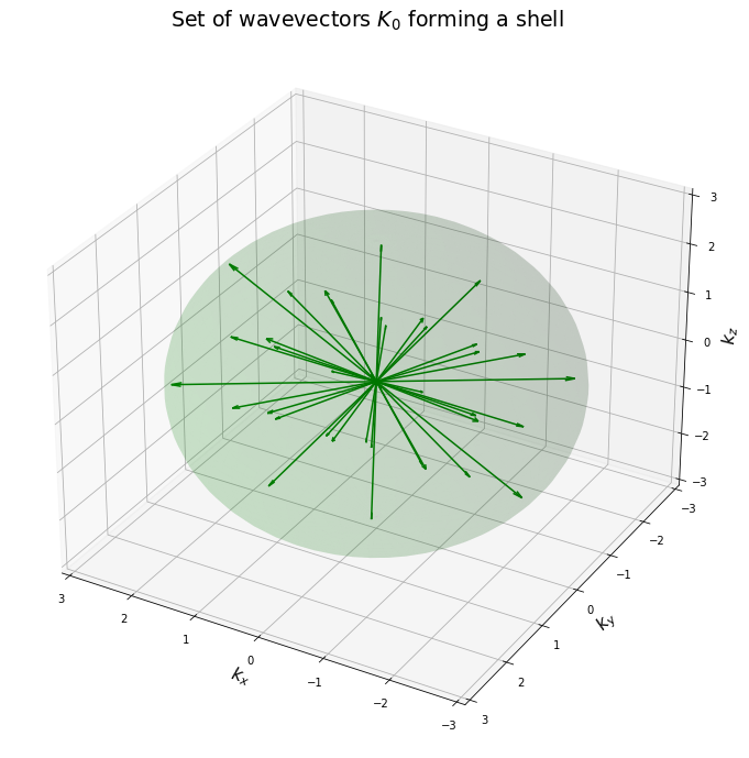
Fig.2 - All wavevectors of the set \(K_0\) spread just enough to approximately form a spherical shell.
In addition, we introduce additional admissible wavevectors by scaling the elements of the \(K_0\) set by a factor of \(2^l\), where l specifies the current shell of these wavevectors. This allows us to define the following sets
\[\begin{align} K_l = \{&\pm 2^l (1.0, 1.0, 1.0),\\ &\pm 2^l (-0.5, 1.0, 1.0),\\ &\pm 2^l (1.0, -0.5, 1.0),\\ &\pm 2^l (1.0, 1.0, -0.5),\\ &\pm 2^l (-0.5, -0.5, 1.0),\\ &\pm 2^l (-0.5, 1.0, -0.5),\\ &\pm 2^l (1.0, -0.5, -0.5),\\ &\pm 2^l (0.5, 2.0, 2.0),\\ &\pm 2^l (2.0, 0.5, 2.0),\\ &\pm 2^l (2.0, 2.0, 0.5),\\ &\pm 2^l (0.5, 0.5, 2.0),\\ &\pm 2^l (0.5, 2.0, 0.5),\\ &\pm 2^l (2.0, 0.5, 0.5),\\ &\pm 2^l (-1.0, 0.5, 2.0),\\ &\pm 2^l (-1.0, 2.0, 0.5),\\ &\pm 2^l (0.5, -1.0, 2.0),\\ &\pm 2^l (0.5, 2.0, -1.0),\\ &\pm 2^l (2.0, -1.0, 0.5),\\ &\pm 2^l (2.0, 0.5, -1.0)\\ &\}. \end{align}\]Each subset \(K_l\) then represents the shell shown in figure 2 but with a radius \(2^l\) higher than the one of \(K_0\). In this way, we can capture a range of spatial scales and partially populate k-space.
Finally, the total set of admissable wavevectors is given by
\[K = \bigcup\limits_{l=0}^{l_{\rm max}} K_l.\]Intra-Shell interactions
Lets clarify how the members of this geometrically scaling set can interact with each other.
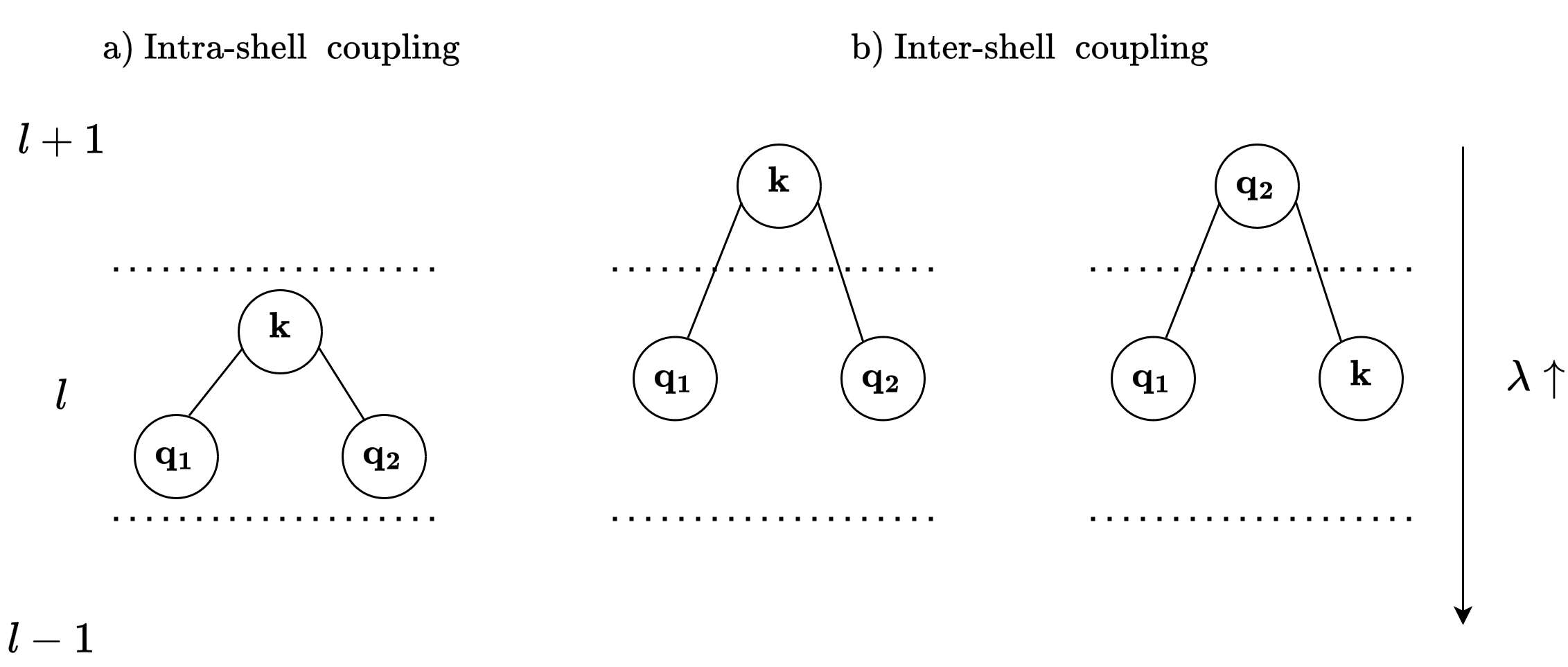
Fig. 3 - Intra- and inter-shell couplings of two Fourier modes with wavevectors \(\mathbf{q}_1\), \(\mathbf{q}_2\) in the REWA model. (a) Intra-shell coupling:
\(\mathbf{q}_1\), \(\mathbf{q}_2\) are in the same shell as the wavevector \(\mathbf{k}\) they couple to. (b) Inter-shell coupling: one of the wavevectors does not lie in the same shell as the other.
Left: \(\mathbf{k}\) does not lie in same shell as the triad participants.
Right: \(\mathbf{k}\) lies in same shell as one of the other wavevectors.
The first type of interaction that can be identified involves triads where two wavevectors, \(\mathbf{q}_1\) and \(\mathbf{q}_2\), couple with a mode whose wavevector \(\mathbf{k}\) lies within the same shell as the initial vectors. Here is an example
\[\underset{\in K_0}{(1,1,1)} + \underset{\in K_0}{(-0.5,1,1)} = \underset{\in K_0}{(0.5,2,2)}.\]Note that these intra-shell interactions involve Fourier modes that correspond to comparable wavelength scales.
Inter-Shell interactions
Another type of interaction occurs when one of the three wavevectors lies in a different shell than the other two. In this case, there a several possible scenarios. It might be that the wavevector \(\mathbf{k}\) that is coupled to is the one that is located in the other shell (see Fig. 3b left). This can include a coupling from lower shells like
\[\underset{\in K_0}{(1,1,1)} + \underset{\in K_0}{(1,1,1)} = \underset{\in K_1}{(2,2,2)},\]or from higher shells like
\[\underset{\in K_1}{(2,-1,-1)} + \underset{\in K_1}{(-1,2,2)} = \underset{\in K_0.}{(1,1,1)}.\]Finally, two wavevectors from different shells can couple to a \(\mathbf{k}\) that resides within the shell of one of the original wavevectors
\[\underset{\in K_0}{(1,1,1)} + \underset{\in K_1}{(2,2,2)} = \underset{\in K_0}{(-1,-1,-1)}.\]The stirring force
As already hinted in part one, the forcing term of the Navier-Stokes equations has yet to be defined. Here we employ a constant stirring force at the largest scales, i.e. in the lowest shell. This force pours energy into the system and keeps the flow going. Energy will of course be removed from the system by dissipation due to viscous effects. Again, we will adapt the term from [1] which is given by
\[\hat{\mathbf{f}}_{\mathbf{k}}(t) = \delta_{\mathbf{k}_0,\mathbf{k}} \frac{\varepsilon}{12} \frac{\hat{\mathbf{u}}_\mathbf{k}(t)}{\sum\limits_{\mathbf{k}_0 \in K_{\rm in}} |\hat{\mathbf{u}}_{\mathbf{k}_0}(t)|},\]where \(K_{\rm in}\) is a subset of \(K_0\) that includes these \(2 \times 6\) wavevectors
\[\begin{align} K_{\rm in} = \{ &\pm (-0.5, 1.0, 1.0),\\ &\pm (1.0, -0.5, 1.0),\\ &\pm (1.0, 1.0, -0.5),\\ &\pm (-0.5, -0.5, 1.0),\\ &\pm (-0.5, 1.0, -0.5),\\ &\pm (1.0, -0.5, -0.5),\\ &\}. \end{align}\]Note that by having \(\mathbf{u}_\mathbf{k}\) appear linearly in the forcing, we have automatically satisfied the divergence-free forcing condition that we assumed during the derivation of the spectral equations of motion, as
\[\mathbf{k} \cdot \hat{\mathbf{f}}_{\mathbf{k}} = 0,\]and hence in real space
\[\nabla \cdot \mathbf{f}(\mathbf{x},t) = 0.\]In the next part of this series, we will also examine the implications of the energy balance associated with this forcing term in more detail.
Implications of the REWA model
In summary, the REWA model limits the number of admissibale wavevectors to a finite subset of, here 38, wavevectors per shell in Fourier space. Figure 4 points out that each shell with index \(l\) corresponds to an eddy of certain spatial extent, given by a wavelength \(\lambda = \frac{2\pi}{|\mathbf{k}|}\). By incorporating multiple shells of finite wavevectors, we create an approximation of the infinite k-space while facilitating interactions between different scales.

Fig. 4 - 2d sketch of the shell model in real space. Higher shells correspond to smaller eddies (wavelengths), while lower lying shells correspond to larger eddies (wavelengths).
While certain interactions are inevitably neglected, this model provides a straightforward method for computing the deterministic chaos of a Newtonian incompressible flow in a fully periodic domain. This will allow us to efficiently explore the phenomenon of turbulence and its properties by numerical simulations.
In the next part of this blog series, we will investigate the energy balances between shell levels and will start to conduct first numerical simulations of the low-order flow model described above to explore the effects it can capture. I believe that simplified models like the REWA offer the greatest insights into physical understanding. I’ll leave you with that, and I’ll see you in the next part.
References
[1] Eggers & Grossmann, Phys. Fluids A 3 (8), 1958 (1991).
[2] Grossmann & Lohse, Phys. Fluids 6, 611 (1994).