Introduction
Loans are a very useful yet sensitive financial product. It is an agreement between two parties, where a lender lends a certain amount of money to a debtor (borrower). In return, the debtor agrees to pay the loan back within a fixed period of time. Furthermore, they will pay an extra sum, called interest, to the lender. This serves as an incentive for the lender to lend the money to the debtor. The latter, on the other hand, can make use of the instant paycheck he or she receives from the lender. In reality, the lender is often a bank, while the borrower might be a private individual who is in need of a certain amount of money to pay for something they cannot afford at the moment.
Taking on a loan can be a very sensitive subject. It feels like living above your standard of living. I grew up with the saying: “If you can’t afford it, you shouldn’t buy it!” While this holds true for taking on a loan to buy a new iPhone, some purchases almost always require one. This might include a car, which you may need to get to work and generate a steady income—especially if public transport is not sufficiently developed in the region where you live. Furthermore, buying property almost always requires a loan as well.
My wife and I took on a loan to buy a car. This was our first experience with “living above our standard of living.” This led me to deepen my basic understanding of loans, and it’s what I want to share in this post.
Deriving some formulas for a loan
Let us start with defining the variables that we need to compute everything we require:
- \(b\) - the credit line, i.e., the amount of money, without interest, you lend from the bank (e.g. \(b=25,000\)€)
- \(r\) - annual or monthly interest rate (e.g. annual interest rate \(r = 5 - 12\%\))
- \(a\) - annual or monthly repayment rate (e.g. monthly repayment rate \(a = 500\)€)
- \(N\) - runtime of the loan, after which the interest and loan have to be paid off
The credit line \(b\) is usually defined by your needs. For example, the car you want to buy might cost 25,000€. Therefore, you ask the bank for a loan of \(b=25,000\)€. Additionally, you know that you can afford to pay back \(500\)€ per month. This obviously depends on your disposable income, i.e., income minus expenses such as rent, food, and so on. The interest rate \(r\) is set by the bank you choose to take the loan from. Besides the reputation of the bank, the interest rate is one of the most important factors when deciding which bank to approach for the loan. Now we will discuss more about the influence of the interest rate on the money you have to repay to the bank below. Moreover, based on these three factors, \(b, a\), and \(r\), the term of the loan can be computed, i.e., the period of time after which your debt to the bank will have decreased to zero, and the loan will be fully paid off.
Now, let us derive a formula that describes the amount of money \(x_n\) you owe the bank after paying an amount \(a\) for \(n\) months. To simplify the notation, let us redefine \(r\) to be the monthly interest rate, that is, the annual interest rate divided by 12. We start with some observations for \(x_0,x_1\), and \(x_2\):
x0=b.
\[x_0 = b.\]Initially, we owe the bank exactly what it lent us: the amount \(b\). Note that it will always be cheapest to pay back the loan instantly, as no interest will accrue. However, this is not an option for us, as otherwise, we wouldn’t need a loan in the first place. Now, let’s see what happens after one month of repaying an amount of \(a\):
\[x_1 = x_0(1+r) - a.\]We have decreased our debt by (a), while the debt has increased by (x_0(1+r)). In the second month, this changes to:
\[x_2 = x_1(1+r) - a = b(1+r)^2 - a(1+r) - a.\]The recursive nature of the formula can already be seen from the first expression. The debt left from the previous month increases through the interest rate, while our repayments decrease it.
Generalizing the observations above leads to the following series:
\[\begin{equation} x_n = x_{n-1}(1+r)-a. \qquad \text{with} \qquad x_0 = b. \end{equation}\]Moreover, we can derive an explicit formula for the current debt depending on \(a,b\), and \(n\), by inserting the recursive formula above for all months. We end up with:
\[x_n = b(1+r)^n - a \sum\limits_{k=0}^{n-1} (1+r)^k= b(1+r)^n - \frac{a}{r}((1+r)^n-1)\]where, in the last step, we made use of the finite geometric series relationship:
\[\sum\limits_{k=m}^n y^k = \frac{y^m - y^{n+1}}{1-y} \qquad \text{where} \qquad y \neq 1.\]This allows us, or rather the bank, to compute a suitable term \(N\) for our loan by setting \(x_N \overset{!}{=} 0\) (after \(N\) months, the loan should be fully paid off). From this, it follows that:
\[N = \left\lceil\frac{\ln\left( \frac{a}{a - rb } \right)}{\ln(1 + r)}\right\rceil,\]where the last repayment in month \(N\) is smaller than the repayment rate \(a\). This is how the bank computes your loan’s term. Of course, the same approach can be used to compute the repayment rate (a) for a fixed term \(N\):
\[a = \frac{rb(1+r)^N}{(1+r)^N-1}.\]Analyzing our results
Let’s plot some figures to visualize what we have derived. We start with the current debt \(x_n\) vs. the current month \(n\) for different annual interest rates \(r\):
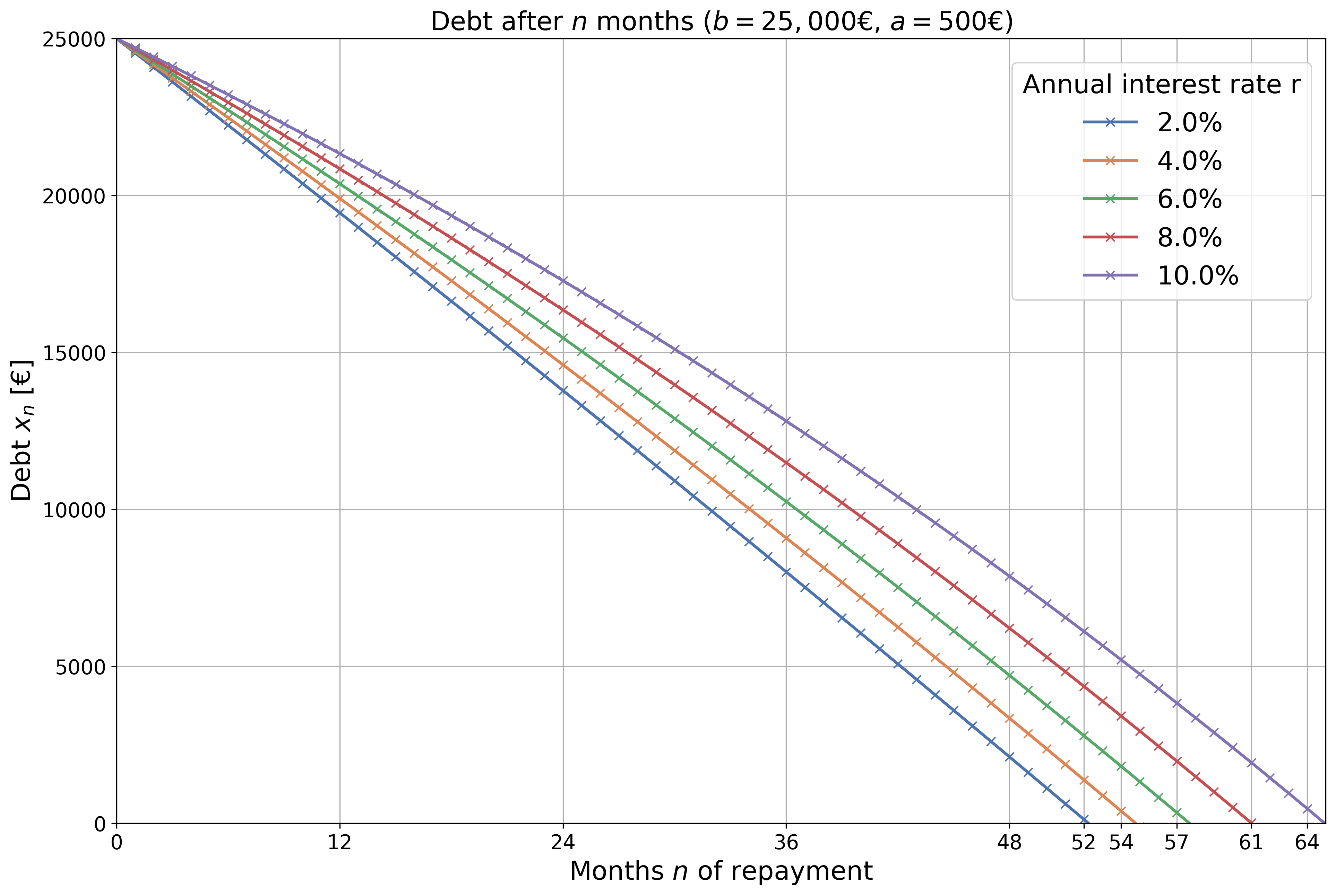
Fig.1 - Scenario for a loan of \(b=25,000\)€ with a monthly repayment rate of \(a=500\)€ for varying interest rates \( r \). It can be seen that for fixed repayment rates, increasing interest rates require increasing loan runtimes.
It can be seen that for small interest rates, the current monthly debt follows an almost linear decrease, while for increasing rates, the trend becomes inherently nonlinear. Furthermore, the runtime increases with \(r\) as the repayment rate stays fixed, and the bank earns more money from your repayment. This can be seen more closely if we take a look at the product \(N a\), which is the total amount of money we pay over the course of the loan’s runtime. It can be decomposed into two components: the amount of money the bank lent us \(b\), and the payment toward interest. This is what we, as debtors to the bank, are most interested in when deciding whether to take the bank’s offer: how “expensive” is my loan?
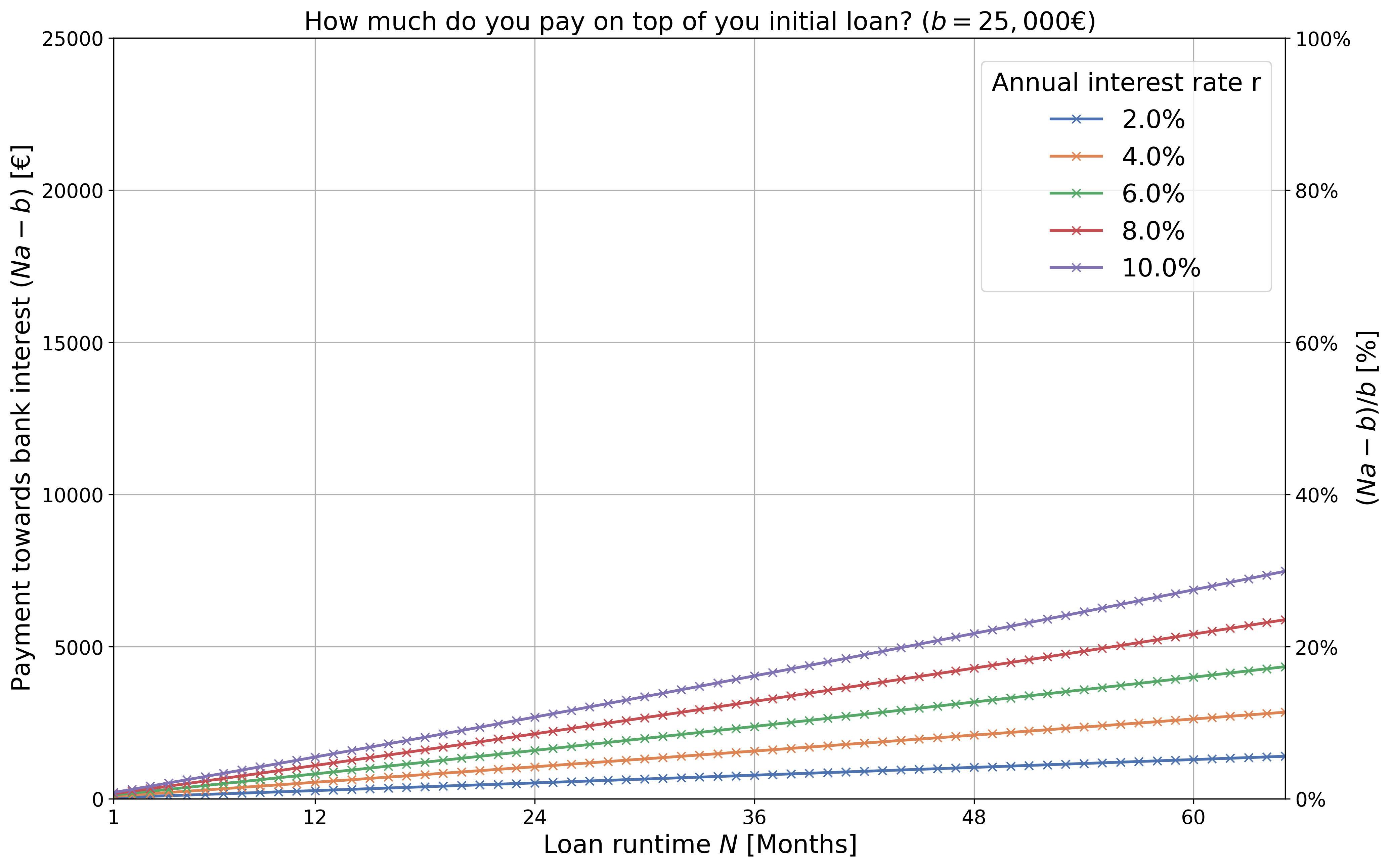
Fig.2 - Increase in payments toward bank interest over the course of the loan runtime and interest rates. A loan of \(b=25,000\)€ was chosen for this example. It can be seen that the longer your loan’s runtime and the higher your interest rates are, the more the bank earns from your loan.
Obviously, longer runtimes and higher interest rates yield more expensive loans. However, how drastically the bank profits from you over longer runtimes is quite alarming. For a 5-year loan with a 10% interest rate, you would need to pay 30% more on top of your credit line. Note that the above graph shows how the annual interest (\(r\)) that we as customers are offered by the banks relates to the overall interest \((Na-b)/b\) over the entire runtime. As we can see, the latter plays in a different league than the former.
In summary: I presented my initial thoughts on loans. It is easy to derive the formulas that might help you understand how banks compute a suitable loan for your needs.
Bonus: Find the bank with the lowest interest rates (again, the bank should be reputable) and try to maximize your monthly payments toward the loan so that the runtime is decreased. Further, try to find loans that allow for unscheduled repayments. This will drastically decrease your payments toward interest!